Continuous time
trajectory estimation for 3D SLAM
from an actuated 2D laser scanner
from an actuated 2D laser scanner
Adrian Haarbach's master's thesis defense
Improved version as of March 28th, 2017
Link to original version from December 19th, 2016
abstract
“ This thesis aims at estimating trajectories for 3D SLAM applications. A continuous time formulation allows solving multiple problems inherent to the traditional discrete time approaches seamlessly, such as sensor fusion of actuated 2D laser scanner data with inertial measurements. Special care is taken when choosing an appropriate trajectory representation. The well-known ICP algorithm used for rigid registration is extended significantly so it can deal with continuous-time, multi-view registration of deformable scans. The resulting algorithm can be employed online in a time-windowed fashion to get an open-loop trajectory estimate and offline for global optimization to further reduce the drift. In contrast to previous work we are able to provide ground truth data for evaluation by extending an existing simulator so that it can simulate actuated 2D laser scanner data with corresponding inertial measurements. Experiments on synthetic data with different scenarios, noise levels and parameter settings show the versatility, stability and adaptability of our algorithm as well as its high overall accuracy.”
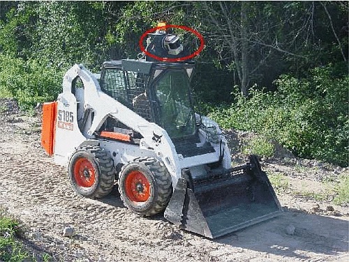
Introduction
stationary 3D scanner
|
actuated 2D scanner
|
Simultaneous Localization And Mapping (SLAM)
Background
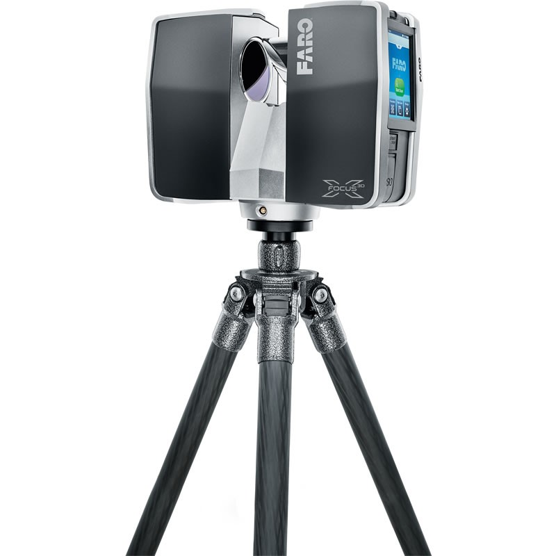
Hardware sensors
LiDAR 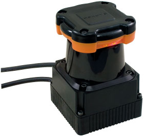 Light Detection And Ranging \( \begin{pmatrix} x \\ y \end{pmatrix} = \begin{pmatrix} r\cos(\phi)\\ r\sin(\phi) \end{pmatrix} \\ \phi = \phi_0 + i\Delta\phi \) |
IMU 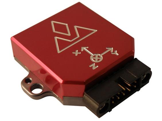 Inertial Measurement Unit \( \newcommand{\angVelMeas}{\base\tilde\angVel\curr & = \base\angVel\curr + \bias_\angVel\curr + \mathcal{N}(\vecb{0},\vecb{\sigma}_\angVel)} \newcommand{\accMeas}{\base\tilde\acc\curr & = \base\acc\curr + \bar{\ori}\curr \gravity + \bias_\acc\curr + \mathcal{N}(\vecb{0},\vecb{\sigma}_\acc)} \begin{align} \angVelMeas &\text{angVel}\\ \accMeas &\text{linAcc} \end{align} \) |
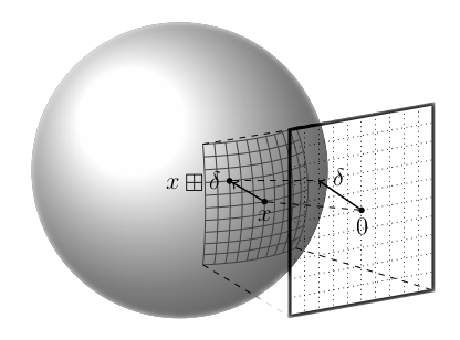
Rotational motion as a manifold
|
Lie group
e.g. rotation matrices \[\mathrm{SO}(3)\] |
 \[\rightleftlie\]
|
Lie algebra
e.g. skew-symmetric matrices \[\mathfrak{so}(3)\] |
unit quaternions
\(\boxed{\SUtwo \cong \spherethree \cong \mathbb{H}_1 = \{\quat \in \mathbb{H} | \norm{\quat} = 1 \}}\)
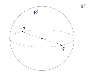
|
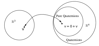
pure quaternions
\(\boxed{\sutwo \cong \rthree \cong \mathbb{H}_0 = \{\quat \in \mathbb{H} | \quatreal = 0 \}} \)
|
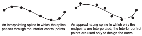
Interpolation
Interpolation vs approximation
Continuity 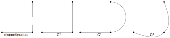
|
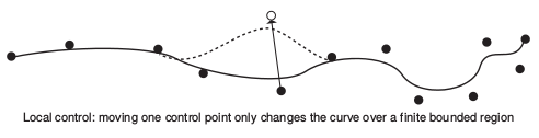
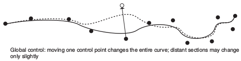
Global vs local control
Complexity LERP, Bezier curve, Bspline |
PCA
Prinical Component Analysis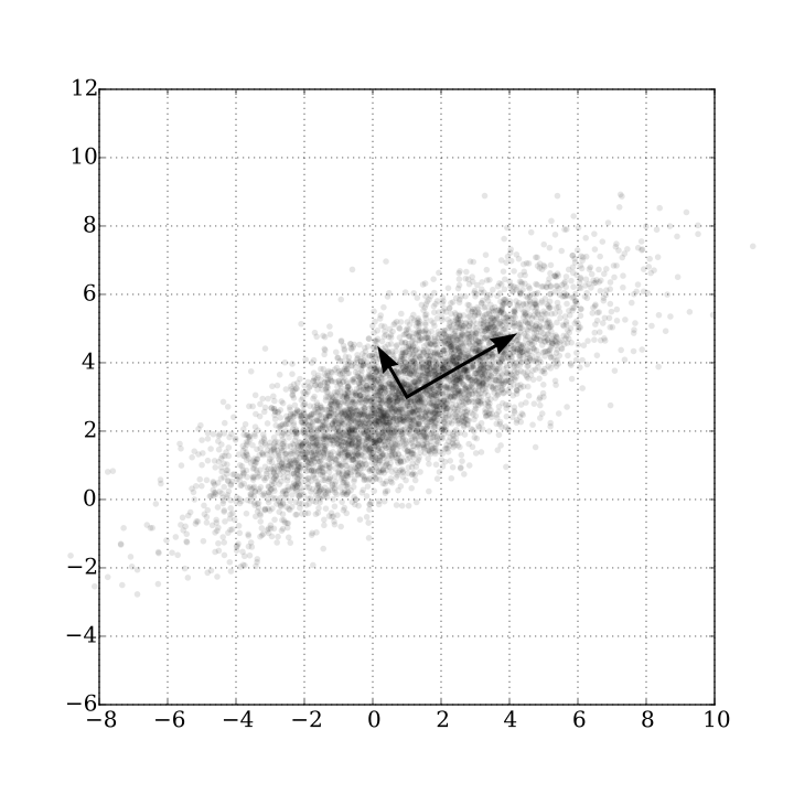
NLS
Non-linear Least Squares: \( E(x) = \factor\sum_{i}^N \left\|f_i\left(x_{i_1}, ... ,x_{i_j}\right)\right\|^2 = \factor\sum_{i=1}^N \res_i^T \res_i = \factor\res^T\res \)Levenberg-Marquardt step:
\( \Delta x = -(J^TJ + \lambda I)^{-1}J^T\res \)
Related work
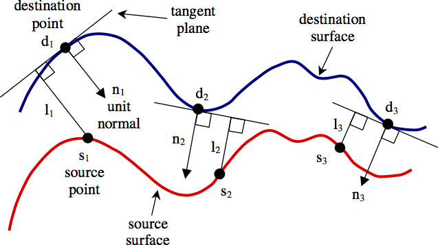
ICP Error Metrics
\(\newcommand{\ppDistFull}{\R\pp_i + \pos - \pq_i} \newcommand{\ppDist}{\vecb{e}_i} %(\pp_i,\pq_i)} \)| point to point | point to plane | plane to plane |
| distance \(\ppDist = \ppDistFull\) | surface normal \(\nq_i\) | modified covariance \(\hat\Cov\) |
| \(E = \sum_{i=1}^N \Norm{\ppDist}^2\) | \( E = \sum_{i=1}^N \Norm{\ppDist \cdot \nq_i }^2\) | \(\newcommand{\gicpInfMatrix}{(\R \hat\Cov_{\pp_i}\R^T + \hat\Cov_{\pq_i})^{-1}} E = \sum_{i=1}^N \ppDist^T \gicpInfMatrix \ppDist \) |
 |
 |
 |
| Besl (1992) Method for registration of 3-d shapes | Chen (1991) Object modeling by registration of multiple range images | Segal (2009) Generalized-ICP |
Actuated 2D lidar
|
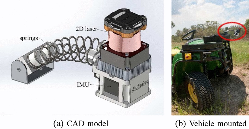 |
|
| Bosse (2009) Continuous 3d scan-matching with a spinning 2d laser | Bosse (2012) Zebedee: Design of a spring- mounted 3-d range sensor... | Kaul (2016) Continuous-time three- dimensional mapping for micro aerial vehicles... |
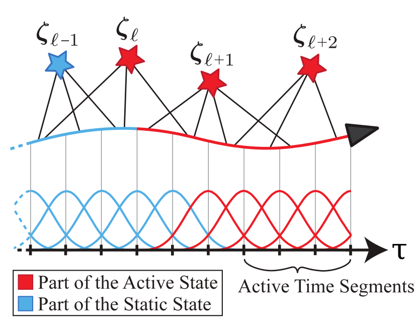
Continuous time estimation
| CT-SLAM | Spline Fusion | CICP |
| high-rate sensors need continuous time SLAM, fewer pose variables | rolling shutter compensation, cumulative B-spline on SE(3) | lidar undistorion, basis B-spline of Cayley-Gibbs-Rodrigues |  |
 |
 |
| Furgale (2012) Continuous-time batch estimation using temporal basis functions | Lovegrove (2013) Spline fusion: A continuous-time representation for visual-inertial fusion... | Alismail (2014) Continuous trajectory estimation for 3d slam from actuated lidar |
Approach
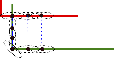
Interpolating orientations
\( \newcommand{\slerpDef}{slerp(\quat_0, \quat_1, u)} \newcommand{\slerp}{\quat_0(\bar{\quat}_0\quat_1)^{u}} \newcommand{\Slerp}{\quat_0 \exp(u\log(\bar{\quat}_0\quat_1))} \slerpDef = \slerp = \Slerp \)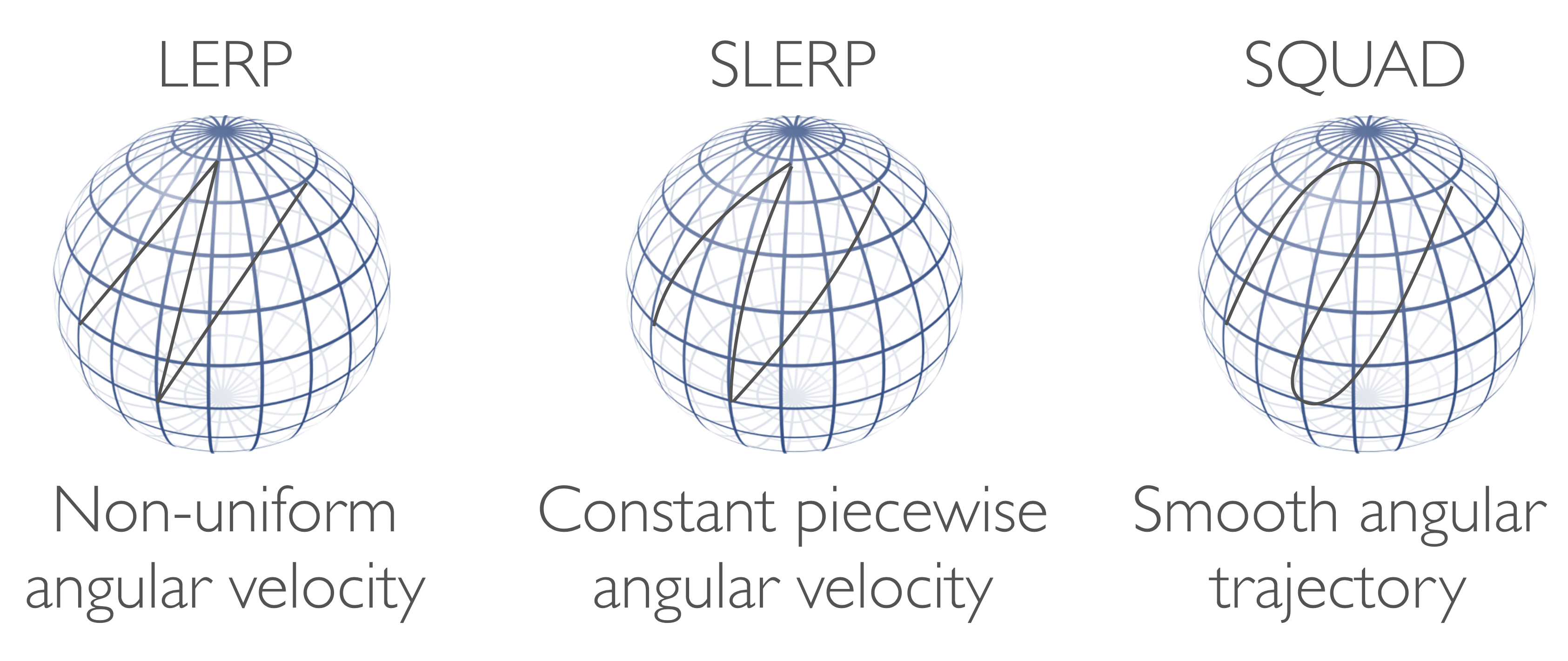
| SLERP: Shoemake (1985) Animating rotation with quaternion curves | SQUAD: Shoemake (1987) Quaternion calculus and fast animation |
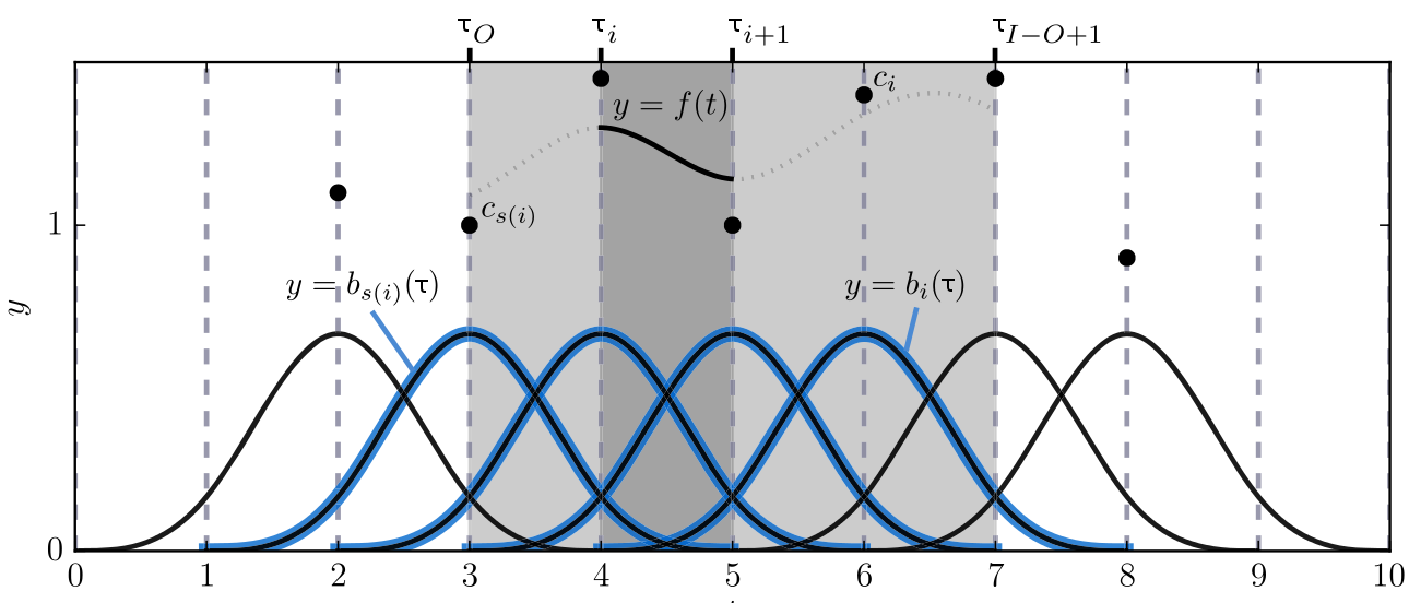
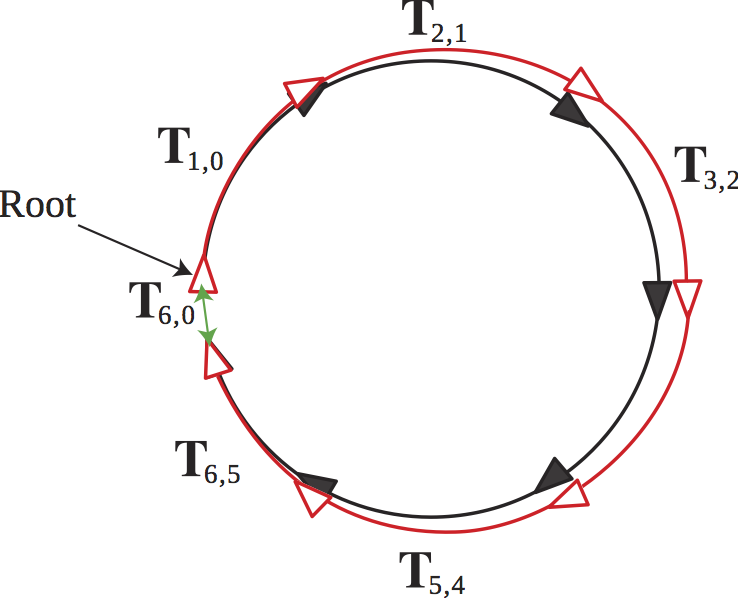
cumulative quaternion B-spline
\( \quat\curr = \quat_0 \prod_{i=1}^n \exp \big( \tilde{N}_i^k\curr \log(\quat_{i-1}^{-1}\quat_{i}) \big) \\ \newcommand{\NC}{ \frac{1}{6} \begin{bmatrix} 0 & 1 & -2 & 1 \\ 0 & -3 & 3 & 0 \\ 0 & 3 & 3 & 0 \\ 6 & 5 & 1 & 0 \end{bmatrix} } \tilde{N}(u) = [u^3, u^2, u, 1] \NC \\ \) Kim (1995) A general construction scheme for unit quaternion curves with simple high order derivatives
Bezier
Slerp
Squad
B-spline
Algorithm
//in: L Lidar scans M IMU measurements
//out: T Trajectory
T = initializeFromIMU(M)
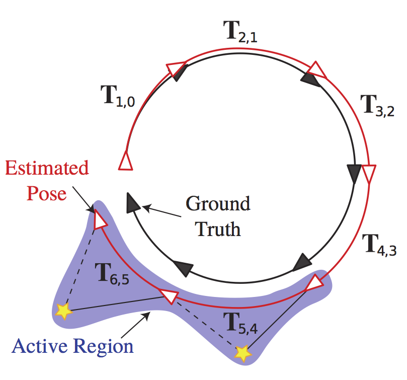
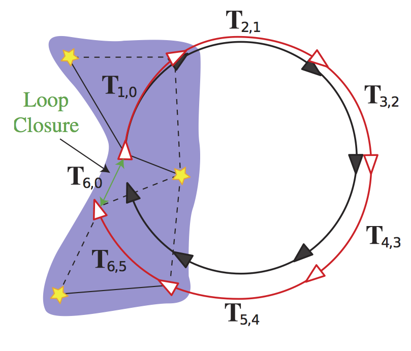
for (i=0 , i < nsweeps , i++ ){
S[i] = unprojectAndAccumulate(L[i*k],...,L[i*k+k])
S[i].undistordAndComputeSurfel(T)
if(i>0){
imuMatches = imuDeviations(T,M[i-1],...,M[i+1])
for (j=0 , j < nicp , j++){
surfelMatches = kdTreeNNLookup(S[i],S[i-1])
T = NLS(T,surfelMatches,imuMatches)
S[i].updateSurfelWorldPositions(T)
}
}
}
\( P(\{\point_i\} \text{ describes plane}) = 2\frac{\eigmiddle-\eigsmall}{\eigsum} \)
imuMatches:
\( \newcommand{\ppDistAbsSurfel}{\bar{d}(a_i,b_i)} \newcommand{\surfelTuple}{(\mean,\normal,\hat\Cov)} \begin{align} \base \eres_\angVel &= \base\tilde\angVel(\timeVar_k) - \base\angVel(\timeVar_k) - \bias_\angVel(\timeVar_k) \\ \base \eres_\acc &= \base\tilde\acc(\timeVar_k) - \bar\quat(\timeVar_k)\gravity - \base\acc(\timeVar_k) - \bias_\acc(\timeVar_k) \end{align} \)
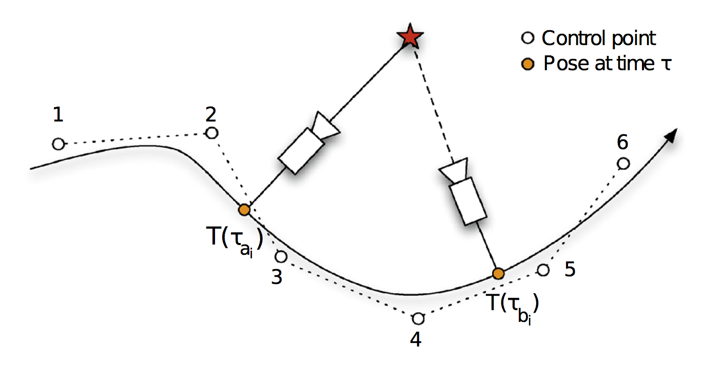
surfelMatches:
\( \begin{align} \ppDistAbsSurfel &= \R_{a_i}\mean_{a_i} + \pos_{a_i} - (\R_{b_i}\mean_{b_i}+\pos_{b_i} )\nonumber \\ \eres_{a_i,b_i} &= \ppDistAbsSurfel^T (\R_h \hat\Cov_{a_i}\R_h^T + \R_k \hat\Cov_{b_i} \R_k^T)^{-1} \ppDistAbsSurfel \\ \\ \end{align} \) combined: \( E = (1-\alpha)\sum_{i=0}^{N} \eres_{a_i,b_i} + \alpha\sum_{j=1}^M\left( \eres_{\angVel_j}^T\Sigma_\angVel^{-1}\eres_{\angVel_j} + \eres_{\acc_j}^T\Sigma_\acc^{-1}\eres_{\acc_j} \right) \)
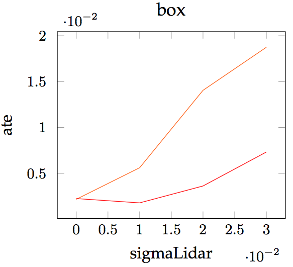
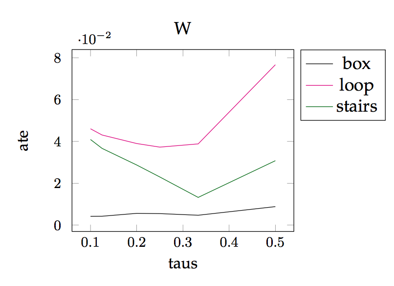
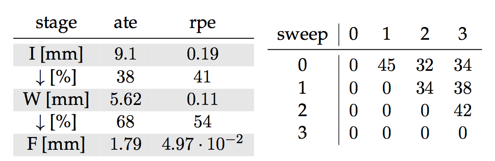
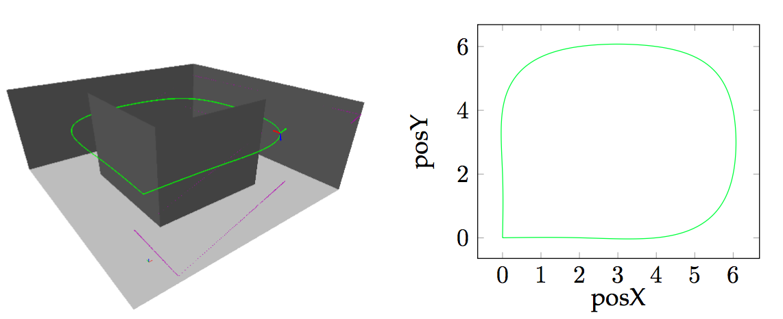
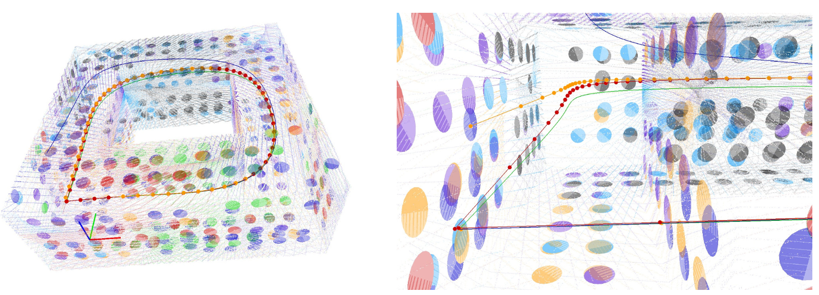
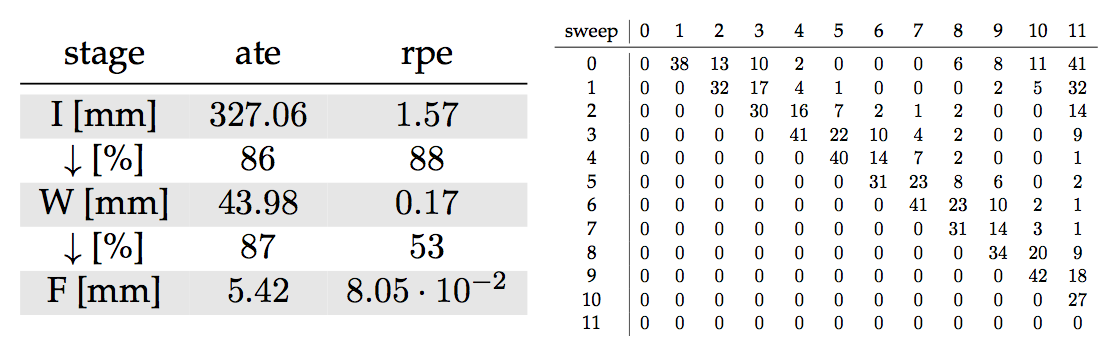
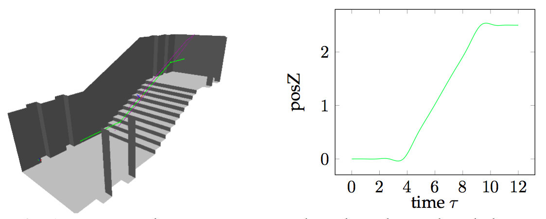
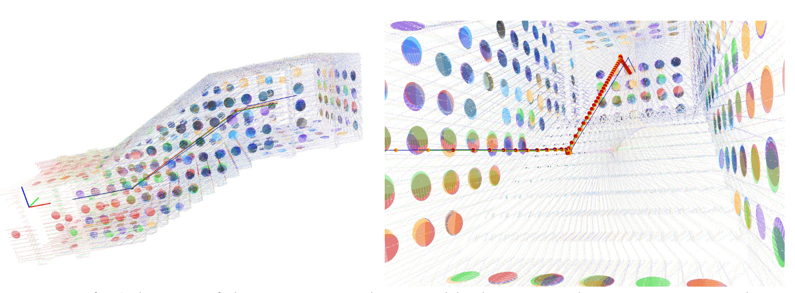
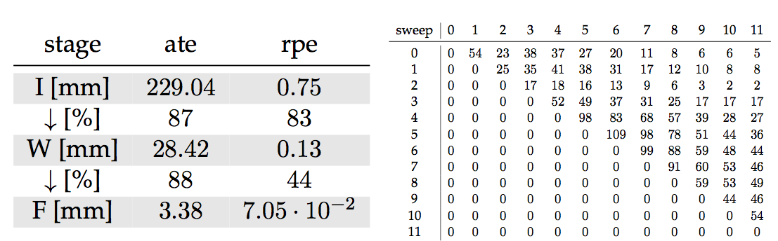
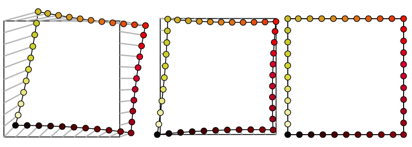
Evaluation